Emissive Participating Media (10pts)
Implementation
Added files:
volpath_ems.cppemissivemedium.cpp
Emissive participating media are heterogeneous media that additionally emit radiance.
To accomplish that they take a second
.vol file as an xml parameter - a temperature grid. By assuming the media is a black body emitter, I
can transform the temperature to emitted radiance via this formula.
To do that, I added a method tempToRadiance() to volumegrid.cpp that converts a temperature to radiance and normalizes the emitted
radiance as describes in PBRv3.
To scale the raw temperature values from the temperature grid, I also added a temp_scale_raw parameter to the xml as well
as a parameter sigma_e that is used to scale the emitted radiance after the temperature has been converted.
To be able to importance sample the emissive medium, I modified the volumegrid.cpp file to additionally compute
a 3D discrete probability distribution in the same spirit as is done for environment map emitters, just with an additional dimension
as we now compute the distribution on voxels and no longer on pixels. This distribution is computed proportional to the luminance
of the individual voxels and can be sampled by calling the sampleGrid() method, which samples
a voxel by sampling 3 individual 1D distributions: $p(x), p(y \ | \ x)$ and $p(z \ | \ y, x)$.
To access the probability of sampling a voxel, I also added a method pdf(). As this sampling is done in index space,
we need to transform the pdf to local medium coordinate space which is done as follows: $p(x_m, y_m, z_m) = p(x_{ind}, y_{ind}, z_{ind}) * \frac{n_x * n_y * n_z}{e_x * e_y * e_z}$,
where $n_i$ denotes the number of grid cells in the i-th dimension and $e_i$ the extents of the bounding box in the i-th dimension.
An emissive medium also offers three additional methods compared to a heterogeneous one. The first one is eval() which does the same thing
as the eval() method of any other emitter: It computes the emitted radiance for a point. It is important that we first need
to transform lRec.p to the local medium coordinate system before we can evaluate the emitted radiance at this point.
The second method is sampleEmission() which calls the sampleGrid() method of the temperature grid and populates
the EmitterQueryRecord. Finally, it returns the emitted radiance divided by the probability of sampling the sampled point. Also here it is important
to transform lRec.p from medium space to world space.
The last method is pdf() that returns the probability of of sampling lRec.p. The probability in local medium
coordinates is obtained by transforming lRec.p to medium space and then calling the pdf() method of the temperature grid. But we now need to transform this probability to solid
angle measure before returning it. I do this in two steps:
-
I divide $pdf_{med}$ by the absolute value of the determinant of the jacobian of
medium_to_world_transform.topLeftCorner(3, 3)to obtain $pdf_{world}$ - I transform $pdf_{world}$ to solid angle measure in the same way as is done for area emitters. For the cosine term I just use 1, as the medium emits the same radiance in to all directions.
Finally, I also added the volpath_ems.cpp integrator, which just does emitter sampling instead of material sampling.
It builds its path by sampling the bsdfs and phase functions but it does not add any contributions from emitters lying on this path (except for direct camera hits).
Instead, it samples a uniformly random light (either a traditional emitter or an emissive medium) at each path vertex and adds its contribution to the radiance accumulator (Light sampling is done similarly as
e.g. in direct_ems). The implementation is pretty similar
to volpath_mats.cpp apart from the difference mentioned above.
Here I also need the intersectTr() method described in the section on heterogeneous media for testing shadowray intersections and obtaining the
the transmittance along the shadowray to attenuate the lights contribution by it. Additionally, the scene now also keeps a list of
all emissive medias to be able to sample from them.
Emissive media are also attached to a mesh and
the xml syntax for specifying an emissive medium is the same as for a heterogeneous one with three additional parameters:
Validation
I validate my implementation by comparing the rendered results for varying parameters and by judging if they look as expected.
I obtained the .vol files by using the converter
offered by mitsuba to convert vdb files which can for example be obtained from here.
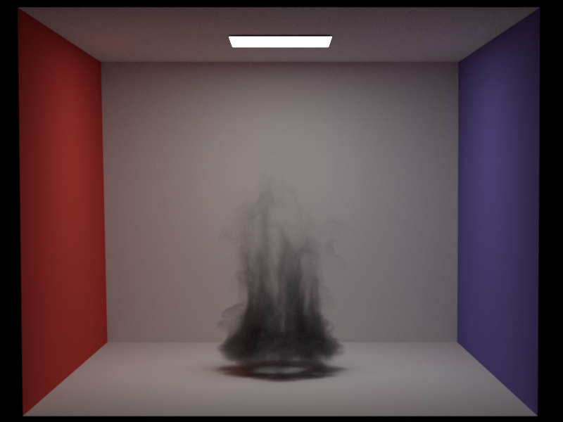
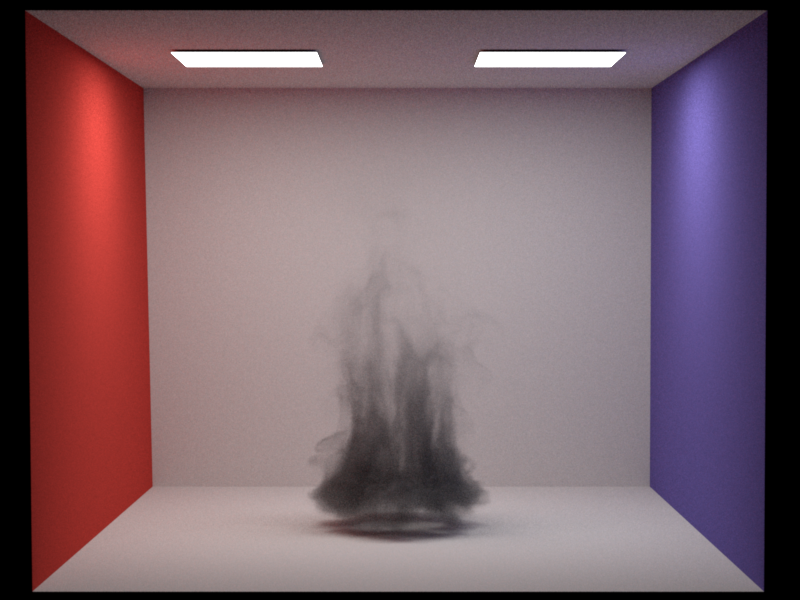
All images were rendered using volpath_mats.cpp unless explicitly stated otherwise.
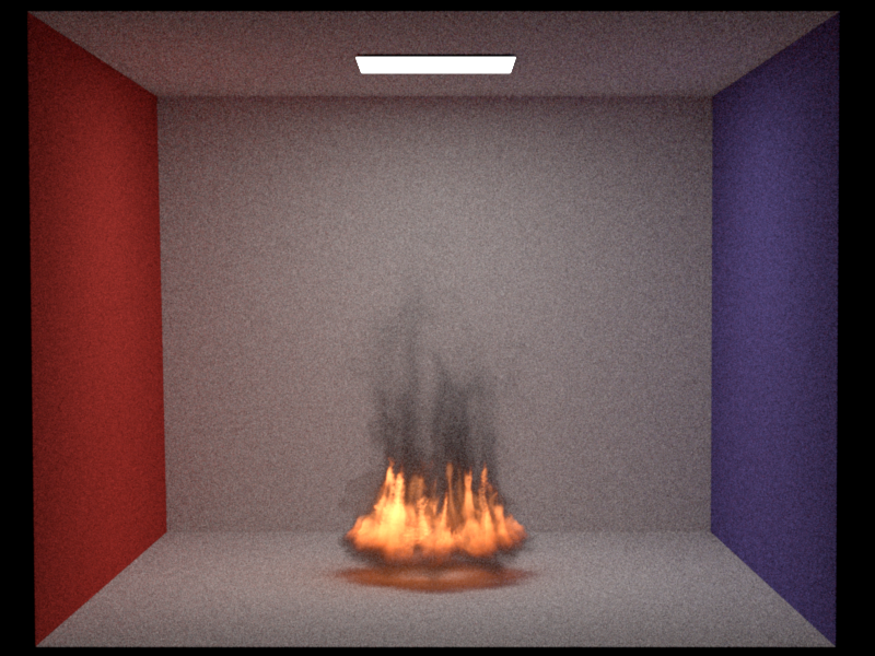
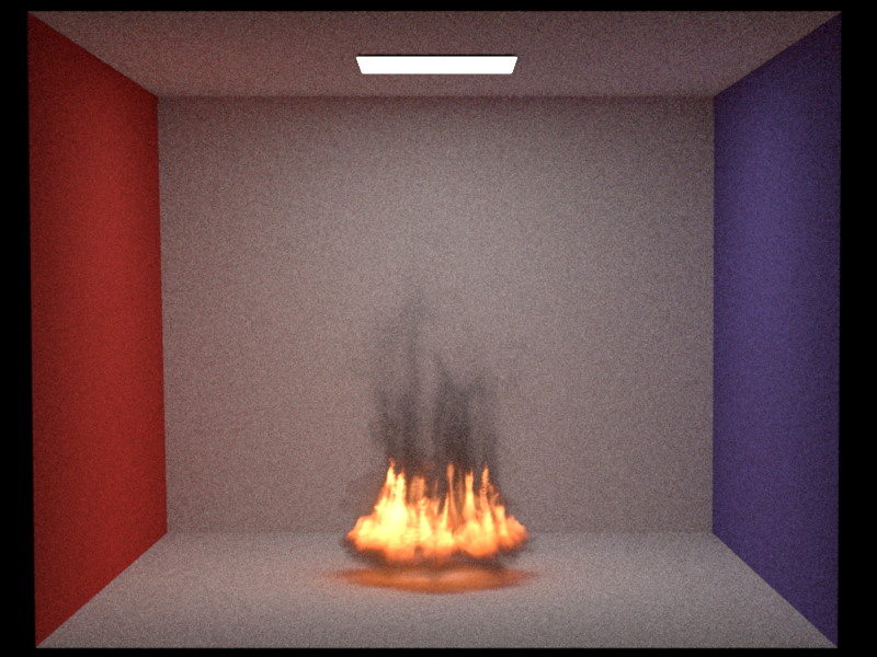
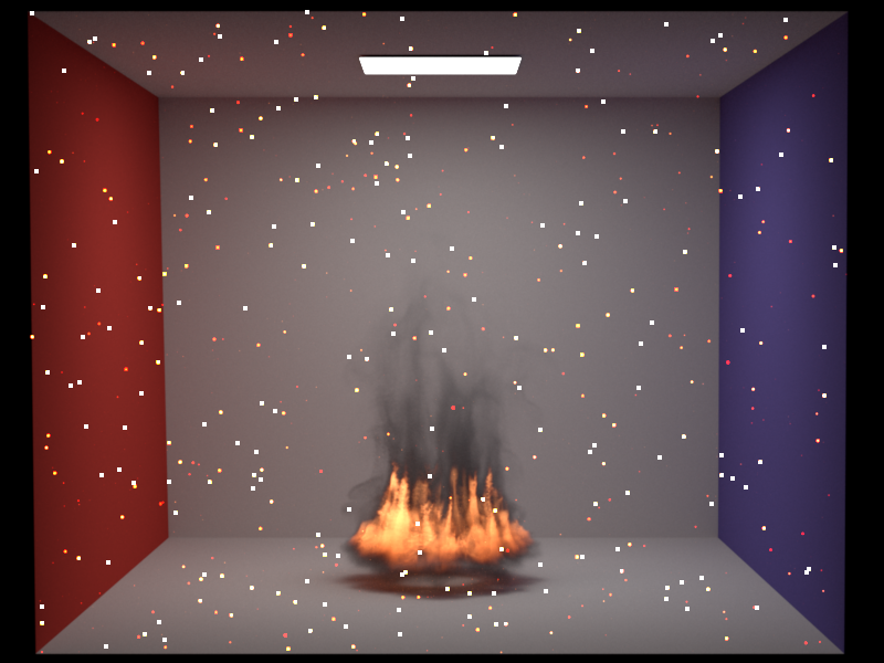
Emissive Medium
The fire rendered looks realistic and one can also see its influence on the environment (e.g. especially below it). Additionally,
varying the parameters does the expected thing.
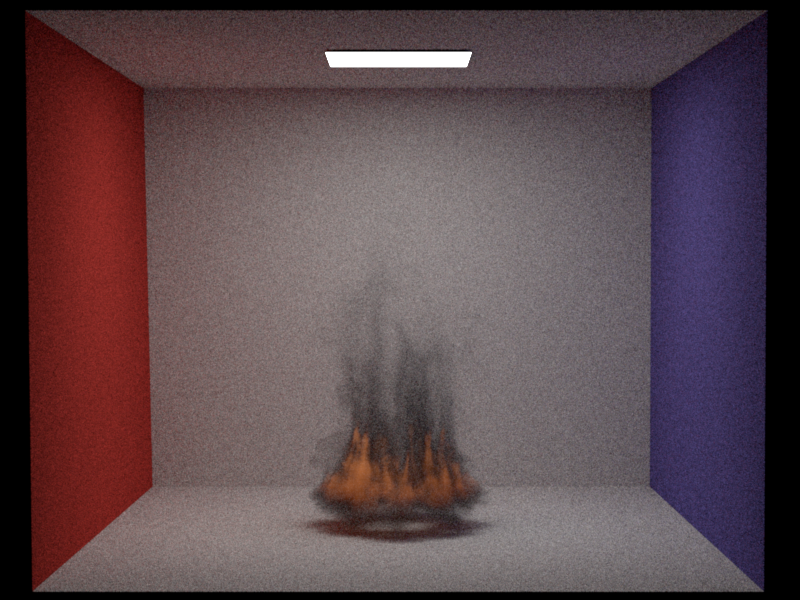
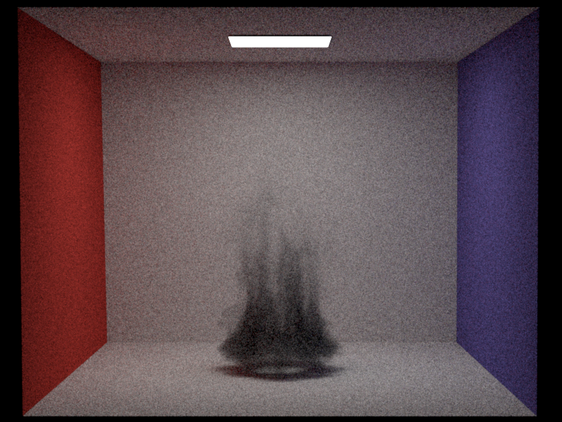
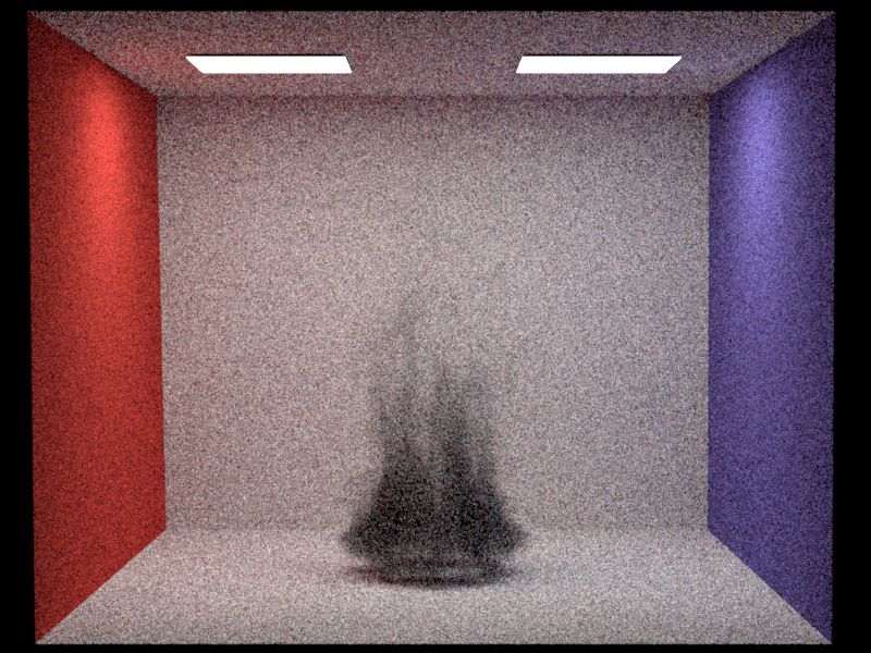
Volpath Ems
I validate volpath_ems.cpp by comparing its renders to the ones from volpath_mats.cpp, as this
integrator was validated by comparing it to other renderers (except for the emissive media part). The results match (except that
the mats integrator has more noise) until
I start adding emissive media to the scene, at which point volpath_ems.cpp starts producing a lot of fireflies
and is darker around the medium than volpath_mats. I assume this is due to an error when converting the
pdf from medium index space to solid angle measure (as without emissive media, the integrators match) which results in
wrong radiance values being added but I did not have enough time to find the issue.
3D discrete probability distribution
As it is hard to visualize a 3D distribution, I compare the computed density (i.e. normalized luminance) to the sampled density (the visualization
is done in the same way as for the environment emitter) for a couple
of fixed z values (where z is the z-index in the voxel grid). The code for creating the images used here can be found
in the precompute() function of volumegrid.cpp.